6 minutes read | published @ January 9, 2015
Gradient Descent Algorithm in Java
How can we make a machine learn from data?
Then, how can we make the machine predicts things based on that learned data? Those are the question answered by one of the most classic Machine Learning Algorithms, the Gradient Descent Algorithm, from a Mathematical-Statistical side it’s called Univariate Linear Regression.
This is one of the tools of the Machine Learning toolbox, and what it tries to do is to model a relationship between a scalar dependent variable Y and a explanatory variable X.
In Layman’s term…
Let’s suppose you have a few points distributed in a Graph, so you already know that in a point A you have a well defined X and Y, which means, if you input X, your output will be Y, and in a point B you have a well defined X’ and Y’ as well. But, thing is, if a point emerge between A and B, and you only have the X… what will be the Y (the output)?
What this algorithm does is: It tries to predict this Y value, based on the previous data! Amazing, right?
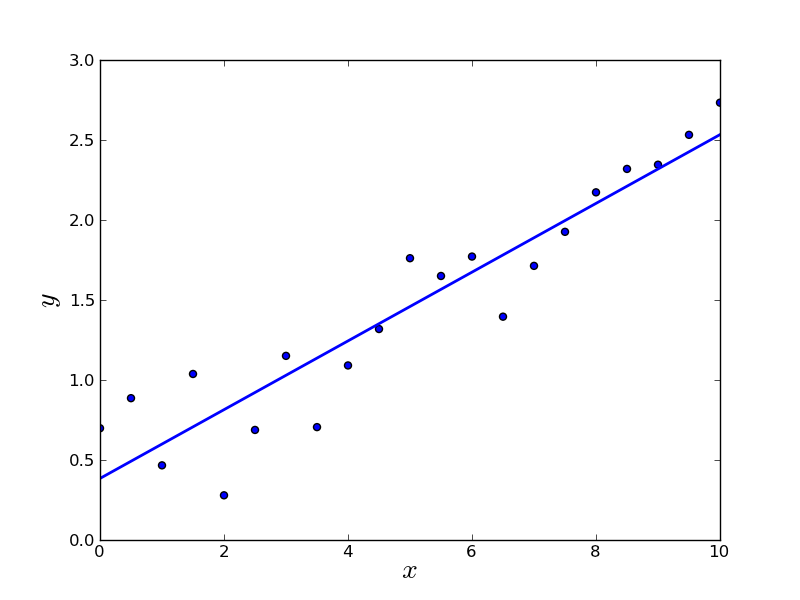
At the end of the execution, you’ll have a full trend line that you can use to predict values! just like the image below.
The Theory Behind It
I’ll cover a few theories about this algorithm here, but, it won’t be complete, as this demand a great coverage of mathematical material that if I would write it all here, It would be a long, long, very long post. So I’m assuming that you’re already familiar with Calculus (Sums, Partial Derivatives), Statistics and Discrete Mathematics.
So, our goal here is to fit the best straight line in our initial data, right?
Thus, we need something to represent this straight line, which will be our hypothesis function:
Where this \( \Theta_{0} \) and \( \Theta_{1} \) are the parameters of the function, and finding the best parameters for this function is what is going to give us the correct straight line to plot on our data.
Here’s an example of what we’re trying to do, which is, fit the best straight line in the data:

So what we want to do is to find a \( \Theta_{0} \) and \( \Theta_{1} \) so our Hypothesis outputs can be very close to the real Y output.
Formally we want:
So we want minimize \( \Theta_{0} \) and \( \Theta_{1} \) so the difference between the Hypothesis and the real output is minimal.
But we want it for every point in our data, which is \(x(i)\) (which is the i-th x of our data), so we want the sum of this average, which is, formally:
And we’re going to call this function Cost Function, with the following notation:
So, our goals is to minimize this cost function:
This cost function is also called Square Error Function.
Now, the gradient descent algorithm
With our cost function built, we need to “keep” finding values for \( \Theta_{0} \) and \( \Theta_{1} \) so we can reach our ideal trend line. So, basically:
1. We start with some \( \Theta_{0} \) and \( \Theta_{1} \)
2. keep changing \( \Theta_{0} \) and \( \Theta_{1} \) to reduce our cost function \( J(\Theta_{0}, \Theta_{1}) \), until we find the minimum.
That’s quite simple and intuitive, right? There’s a lot of intuitive explanation and more visual examples of what this algorithm is doing in the machine learning course taught by Andrews Ng (From Stanford).
What this algorithm will be doing is: partially derive our cost function for \( \Theta_{0} \) and \( \Theta_{1} \) simultaneously, so we can find the minimum value for them, with every iteration updating our \( \Theta_{0} \) and \( \Theta_{1} \) with their new value!
Meh, talk is cheap show me the math!
Formally, the algorithm is:
Make sure that this will run for j = 0 and j = 1.
But, pay attention, this is the generic version, the \( \Theta_{j} \) represent both \( \Theta_{0} \) and \( \Theta_{1} \).
What the algorithm is saying is that we’ll be doing this procedure to \( \Theta_{0} \) and \( \Theta_{1} \) at the same time! So, we can put it in this way:
Also, we can expand the Cost Function that is being derived, doing this, it will be exactly what I’ll be putting into code soon, so, our final algorithm is:
Now it’s time to code all of it!
First things first, we’ll be using Google’s JMathPlot to plot graphs using Java and Swing to use its JFrame, we shall start with our class to represent our Initial Data, which will be the Training Set.

Now we’re going to take our first steps on writing the GradientDescent.java, we must be very careful here. Let’s start with the main settings and parameters of it:
Now let me explain a few details of this part:
Alpha is the Learning Rate, it’s a dangerous variable, it’s used to set the size of the step that the algorithm will take while trying to find the \( \Theta_{0} \) and \( \Theta_{1} \), that’s the learning rate of the algorithm. If Alpha is too low, the algorithm can be very slow, although very precise, if Alpha is higher, it will be taking larger steps, which can be faster, or dangerous, causing the algorithm to DIVERGE, which, trust me, you don’t want this! (Andrew Ng explain this part very well in its course)
The variable TrendLine is what we’ll use to plot the straight line which is our main goal.
The tol variable is our safe move in case of a dangerous convergence, which means, in case of convergence, it will stop the execution.
The other variables and objects in this part are very intuitive to understand, it’s auto explainable! (forgive if i’m wrong, just say something and I’ll put more detail on that).
About the Constructor, we’re saying that our initial guesses for \( \Theta_{0} \) and \( \Theta_{1} \) is 0. The rest is just data plotting.
next: our Hypothesis Function (that will be doing exactly as the model that I did show above)
Now, our two function to derive our \( \Theta \), again, it will be doing exactly the same as the mathematical model, there’s no magic!
Note that it does almost exactly the same as the mathematical model of the Gradient Descent demonstrated above, the difference is only a few details, such as the if and while to verify convergence or divergence (which is, if it reached the iteration’s limit)
Next we have the addTrendLine function, used to keep plotting our straight line as it will become more updated.
And now we have an extra, it’s a function to store and plot the convergence history of both \( \Theta_{0} \) and \( \Theta_{1} \), so we can see how it happened.
Finally, we have our Test Class, that will execute everything:
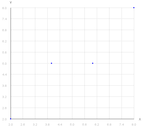
Now, executing the code, the output will be, at first, the initial data:
Executing the algorithm, it learns and generate its prediction based on its initial data:
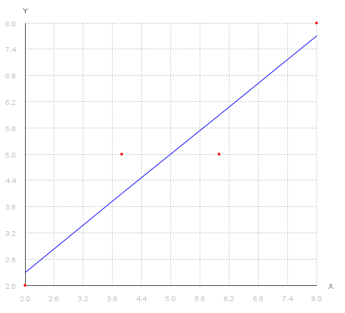
Magical, right?
And then, we can see the convergence:
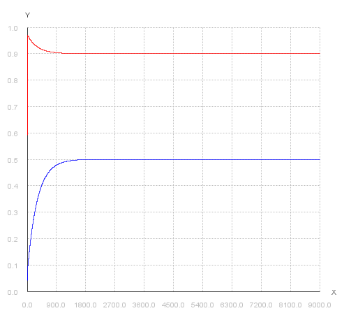
And you can see in the terminal the final values of \( \Theta_{0} \) and \( \Theta_{1} \) that minimized the Cost Function.
If it wasn’t Science, probably would be black magic. heh.
A few considerations
You can download the complete code here.
If you have any questions/suggestion, drop me an email so we can talk!
If you need further details of the mathematical model, I ultra advice to watch Andrew’s Ng Videos at Stanford@Coursera. His skills to teach it is something unbelievable awesome.
Thanks for reading!
machine learningartificial intelligencejavaprogrammingengineeringtutorial
1274 Words
2015-01-09 00:00 +0000
8bd269c @ 2020-02-08